Usage
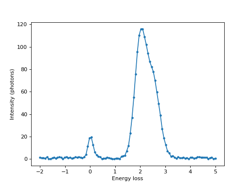
RIXS spectra at SIX are represented as two-column arrays of values, where the axes are energy loss and intensity. If we call such as spectrum S, it can be plotted by
import matplotlib.pyplot as plt
fig, ax = plt.subplots()
ax.plot(S[:,0], S[:,1])
The use of BlueSky at SIX allows us to take RIXS spectra at a series of different conditions in a single operation or scan. For example one could vary the scattering angle \(\theta\) to measure at low, medium and high \(\theta\). The scan containing all spectra is retrieved via
from sixtools.rixswrapper import make_scan
from databroker in DataBroker as db

scan = make_scan(db[21110])
scan is then a 4D numpy array. Its axes are:
axis 0 – event in scan
axis 1 – frame in event
axis 2 – row in spectrum
axis 3 – axis of spectrum
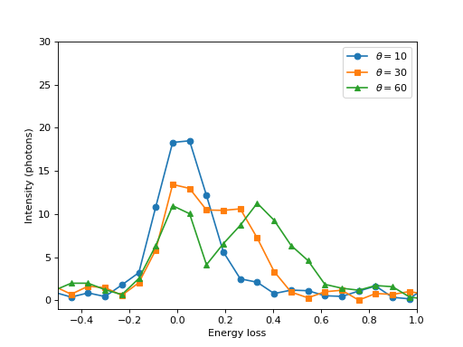
Since each frame is taken under nominally the same conditions (i.e. the same \(\theta\) in our example), one might want to add the spectra at each event.
scan_events_summed = scan.sum(axis=1)
These summed spectra could be plotted by against \(\theta\), which we can read out of the databroker. Let’s zoom on the low energy region, as this is more likely to be dispersive.
fig, ax  = plt.subplots()

thetas = db[21110].table(fields=['theta'])

for S, theta in zip(scan_events_summed, thetas):
    ax.plot(S[:,0], S[:,1], label='$\theta={}$'.format(theta))
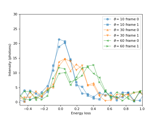
or alternatively one can plot all individual spectra
import matplotlib.pyplot as plt
fig, ax  = plt.subplots()

for event, theta in zip(scan, theta):
    for frame_ind, S in enumerate(event):
        ax.plot(S[:,0], S[:,1],
        label='$\theta={} frame {}'.format(theta, frame_ind))
Powerful numpy broadcasting methods can be used to manipulate the whole scan at once. See Numpy documentation or the calibrate function in sixtools.rixswrapper.